Scikit-learn hyperparameter search wrapper

Iaroslav Shcherbatyi, Tim Head and Gilles Louppe. June 2017. Reformatted by Holger Nahrstaedt 2020

Introduction

This example assumes basic familiarity with scikit-learn.

Search for parameters of machine learning models that results in best cross-validation performance is necessary in almost all practical cases to get a model with best generalization estimate. A standard approach in scikit-learn is to use sklearn.model_selection.GridSearchCV class, which enumerates all combinations of hyperparameters values given as input. This search complexity grows exponentially with the number of parameters. A more scalable approach is to use sklearn.model_selection.RandomizedSearchCV, which however does not take advantage of the structure of a search space. Scikit-optimize provides a drop-in replacement for these two scikit-learn methods. The hyperparameter search is achieved by Bayesian Optimization At each step of the optimization, a surrogate model infers the objective function using observed evluation results as priors. An acquisition function utilizes these predictions to navigate between exploration (sampling unexplored areas) and exploitation (focusing on regions likely containing the global optimum). By balancing these two strategies, Bayesian Optimization identifies probable optimal areas while ensuring comprehensive search coverage. In practice, this method often leads to quicker and better results.

Note: for a manual hyperparameter optimization example, see “Hyperparameter Optimization” notebook.

print(__doc__)
import numpy as np

np.random.seed(123)
import matplotlib.pyplot as plt
from sklearn.datasets import load_digits
from sklearn.model_selection import train_test_split
from sklearn.svm import SVC

from skopt import BayesSearchCV

Minimal example

A minimal example of optimizing hyperparameters of SVC (Support Vector machine Classifier) is given below.

X, y = load_digits(n_class=10, return_X_y=True)
X_train, X_test, y_train, y_test = train_test_split(
    X, y, train_size=0.75, test_size=0.25, random_state=0
)

# log-uniform: understand as search over p = exp(x) by varying x
opt = BayesSearchCV(
    SVC(),
    {
        'C': (1e-6, 1e6, 'log-uniform'),
        'gamma': (1e-6, 1e1, 'log-uniform'),
        'degree': (1, 8),  # integer valued parameter
        'kernel': ['linear', 'poly', 'rbf'],  # categorical parameter
    },
    n_iter=32,
    cv=3,
)

opt.fit(X_train, y_train)

print("val. score: %s" % opt.best_score_)
print("test score: %s" % opt.score(X_test, y_test))

val. score: 0.9866369710467705
test score: 0.9844444444444445

Advanced example

In practice, one wants to enumerate over multiple predictive model classes, with different search spaces and number of evaluations per class. An example of such search over parameters of Linear SVM, Kernel SVM, and decision trees is given below.

from sklearn.datasets import load_digits
from sklearn.model_selection import train_test_split
from sklearn.pipeline import Pipeline
from sklearn.svm import SVC, LinearSVC

from skopt import BayesSearchCV
from skopt.plots import plot_histogram, plot_objective
from skopt.space import Categorical, Integer, Real

X, y = load_digits(n_class=10, return_X_y=True)
X_train, X_test, y_train, y_test = train_test_split(X, y, random_state=0)

# pipeline class is used as estimator to enable
# search over different model types
pipe = Pipeline([('model', SVC())])

# single categorical value of 'model' parameter is
# sets the model class
# We will get ConvergenceWarnings because the problem is not well-conditioned.
# But that's fine, this is just an example.
linsvc_search = {
    'model': [LinearSVC(max_iter=1000, dual="auto")],
    'model__C': (1e-6, 1e6, 'log-uniform'),
}

# explicit dimension classes can be specified like this
svc_search = {
    'model': Categorical([SVC()]),
    'model__C': Real(1e-6, 1e6, prior='log-uniform'),
    'model__gamma': Real(1e-6, 1e1, prior='log-uniform'),
    'model__degree': Integer(1, 8),
    'model__kernel': Categorical(['linear', 'poly', 'rbf']),
}

opt = BayesSearchCV(
    pipe,
    # (parameter space, # of evaluations)
    [(svc_search, 40), (linsvc_search, 16)],
    cv=3,
)

opt.fit(X_train, y_train)

print("val. score: %s" % opt.best_score_)
print("test score: %s" % opt.score(X_test, y_test))
print("best params: %s" % str(opt.best_params_))

val. score: 0.9881217520415739
test score: 0.9888888888888889
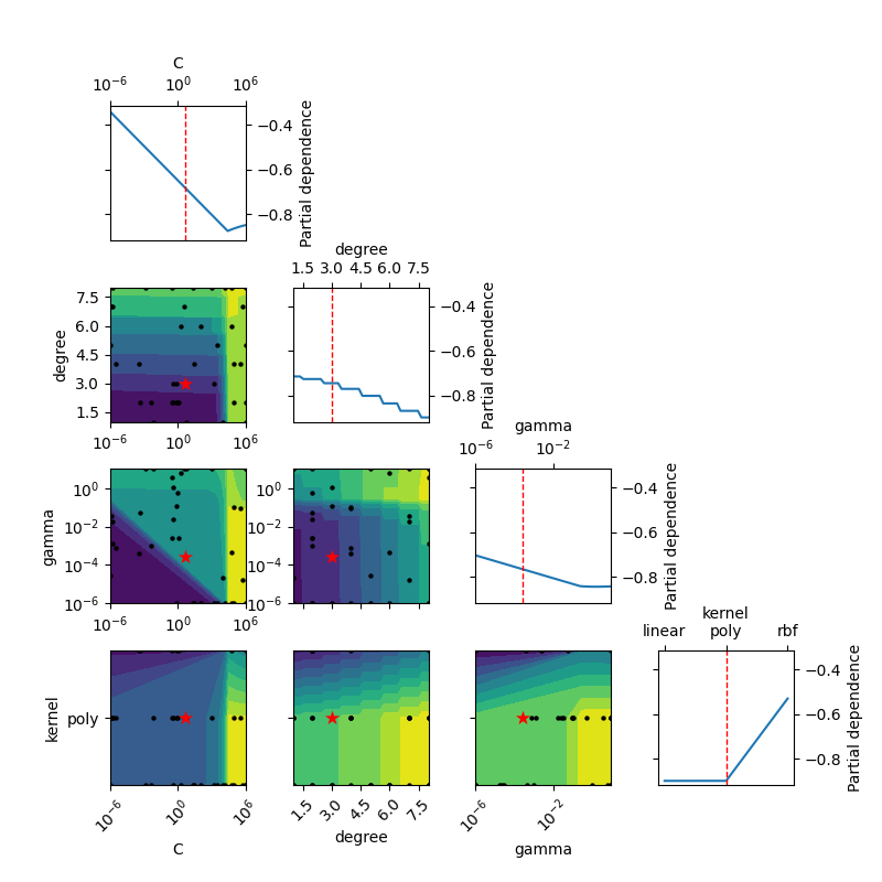
best params: OrderedDict([('model', SVC()), ('model__C', 4.580543393203649), ('model__degree', 3), ('model__gamma', 0.0002585937465230229), ('model__kernel', 'poly')])

Partial Dependence plot of the objective function for SVC

_ = plot_objective(
    opt.optimizer_results_[0],
    dimensions=["C", "degree", "gamma", "kernel"],
    n_minimum_search=int(1e8),
)
plt.show()

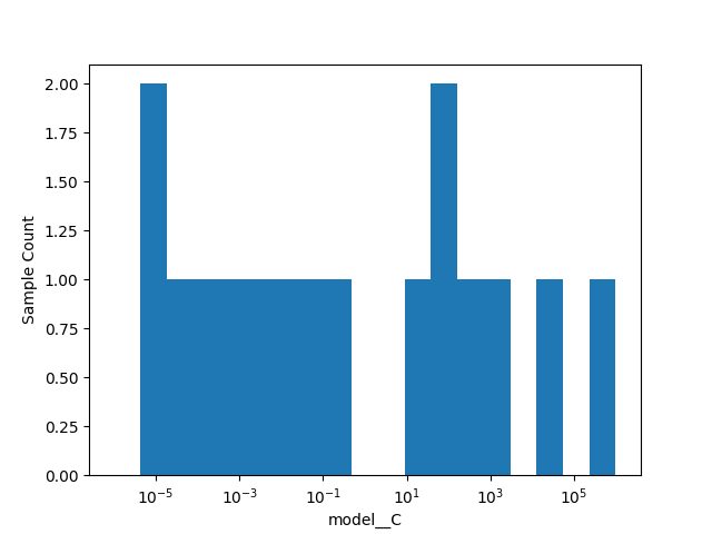
Plot of the histogram for LinearSVC

_ = plot_histogram(opt.optimizer_results_[1], 1)
plt.show()

Progress monitoring and control using callback argument of fit method

It is possible to monitor the progress of BayesSearchCV with an event handler that is called on every step of subspace exploration. For single job mode, this is called on every evaluation of model configuration, and for parallel mode, this is called when n_jobs model configurations are evaluated in parallel.

Additionally, exploration can be stopped if the callback returns True. This can be used to stop the exploration early, for instance when the accuracy that you get is sufficiently high.

An example usage is shown below.

from sklearn.datasets import load_iris
from sklearn.svm import SVC

from skopt import BayesSearchCV

X, y = load_iris(return_X_y=True)

searchcv = BayesSearchCV(
    SVC(gamma='scale'),
    search_spaces={'C': (0.01, 100.0, 'log-uniform')},
    n_iter=10,
    cv=3,
)


# callback handler
def on_step(optim_result):
    score = -optim_result['fun']
    print("best score: %s" % score)
    if score >= 0.98:
        print('Interrupting!')
        return True


searchcv.fit(X, y, callback=on_step)

best score: 0.98
Interrupting!

BayesSearchCV(cv=3, estimator=SVC(), n_iter=10,
              search_spaces={'C': (0.01, 100.0, 'log-uniform')})

In a Jupyter environment, please rerun this cell to show the HTML representation or trust the notebook.
On GitHub, the HTML representation is unable to render, please try loading this page with nbviewer.org.

Counting total iterations that will be used to explore all subspaces

Subspaces in previous examples can further increase in complexity if you add new model subspaces or dimensions for feature extraction pipelines. For monitoring of progress, you would like to know the total number of iterations it will take to explore all subspaces. This can be calculated with total_iterations property, as in the code below.

from sklearn.datasets import load_iris
from sklearn.svm import SVC

from skopt import BayesSearchCV

X, y = load_iris(return_X_y=True)

searchcv = BayesSearchCV(
    SVC(),
    search_spaces=[
        ({'C': (0.1, 1.0)}, 19),  # 19 iterations for this subspace
        {'gamma': (0.1, 1.0)},
    ],
    n_iter=10,
)

print(searchcv.total_iterations)

29