Use different base estimators for optimization

Sigurd Carlen, September 2019. Reformatted by Holger Nahrstaedt 2020

To use different base_estimator or create a regressor with different parameters, we can create a regressor object and set it as kernel.

This example uses plots.plot_gaussian_process which is available since version 0.8.

print(__doc__)

import numpy as np

np.random.seed(1234)
import matplotlib.pyplot as plt

from skopt import Optimizer
from skopt.plots import plot_gaussian_process

Toy example

Let assume the following noisy function \(f\):

noise_level = 0.1

# Our 1D toy problem, this is the function we are trying to
# minimize


def objective(x, noise_level=noise_level):
    return np.sin(5 * x[0]) * (1 - np.tanh(x[0] ** 2)) + np.random.randn() * noise_level


def objective_wo_noise(x):
    return objective(x, noise_level=0)

opt_gp = Optimizer(
    [(-2.0, 2.0)],
    base_estimator="GP",
    n_initial_points=5,
    acq_optimizer="sampling",
    random_state=42,
)

def plot_optimizer(res, n_iter, max_iters=5):
    if n_iter == 0:
        show_legend = True
    else:
        show_legend = False
    ax = plt.subplot(max_iters, 2, 2 * n_iter + 1)
    # Plot GP(x) + contours
    ax = plot_gaussian_process(
        res,
        ax=ax,
        objective=objective_wo_noise,
        noise_level=noise_level,
        show_legend=show_legend,
        show_title=True,
        show_next_point=False,
        show_acq_func=False,
    )
    ax.set_ylabel("")
    ax.set_xlabel("")
    if n_iter < max_iters - 1:
        ax.get_xaxis().set_ticklabels([])
    # Plot EI(x)
    ax = plt.subplot(max_iters, 2, 2 * n_iter + 2)
    ax = plot_gaussian_process(
        res,
        ax=ax,
        noise_level=noise_level,
        show_legend=show_legend,
        show_title=False,
        show_next_point=True,
        show_acq_func=True,
        show_observations=False,
        show_mu=False,
    )
    ax.set_ylabel("")
    ax.set_xlabel("")
    if n_iter < max_iters - 1:
        ax.get_xaxis().set_ticklabels([])

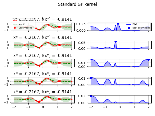
GP kernel

fig = plt.figure()
fig.suptitle("Standard GP kernel")
for i in range(10):
    next_x = opt_gp.ask()
    f_val = objective(next_x)
    res = opt_gp.tell(next_x, f_val)
    if i >= 5:
        plot_optimizer(res, n_iter=i - 5, max_iters=5)
plt.tight_layout(rect=[0, 0.03, 1, 0.95])
plt.plot()

[]

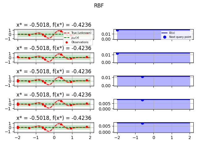
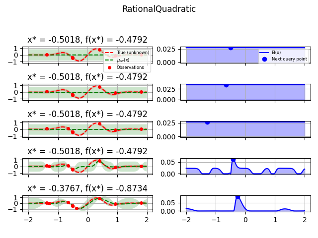
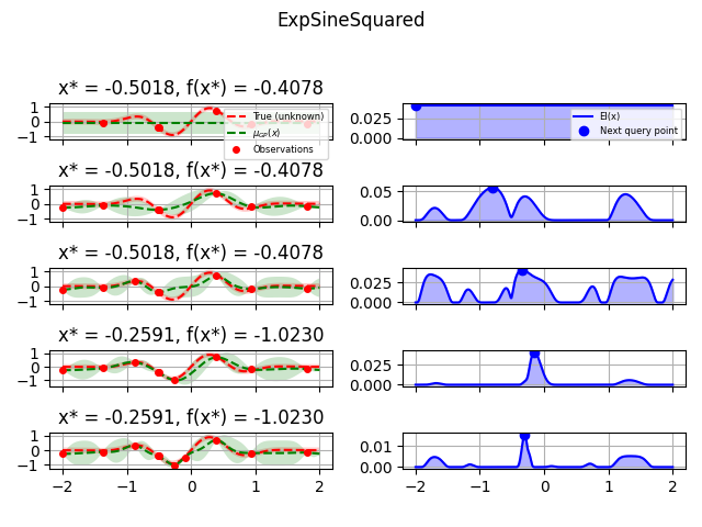
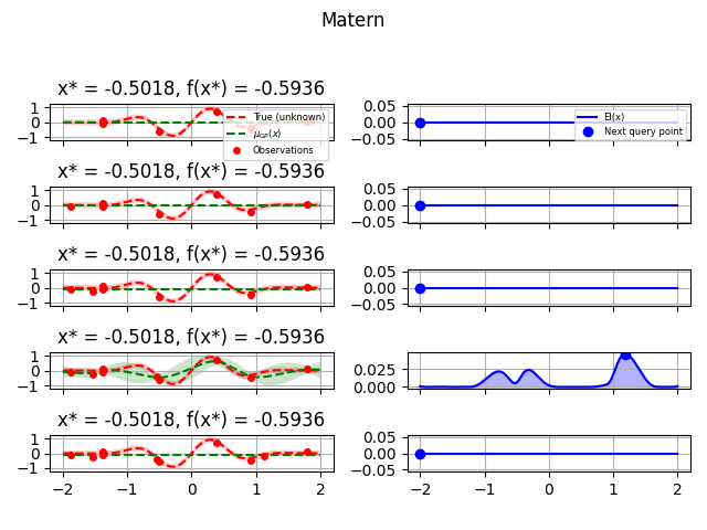
Test different kernels

from sklearn.gaussian_process.kernels import (
    RBF,
    ConstantKernel,
    DotProduct,
    ExpSineSquared,
    Matern,
    RationalQuadratic,
)

from skopt.learning import GaussianProcessRegressor
from skopt.learning.gaussian_process.kernels import ConstantKernel, Matern

# Gaussian process with Matérn kernel as surrogate model


kernels = [
    (1.0 * RBF(length_scale=1.0, length_scale_bounds=(1e-1, 10.0)), "RBF"),
    (1.0 * RationalQuadratic(length_scale=1.0, alpha=0.1), "RationalQuadratic"),
    (1.0
    * ExpSineSquared(
        length_scale=1.0,
        periodicity=3.0,
        length_scale_bounds=(0.1, 10.0),
        periodicity_bounds=(1.0, 10.0),
    ), "ExpSineSquared"),
    # (ConstantKernel(0.1, (0.01, 10.0))
    # * (DotProduct(sigma_0=1.0, sigma_0_bounds=(0.1, 10.0)) ** 2), "ConstantKernel"),
    (1.0 * Matern(length_scale=1.0, length_scale_bounds=(1e-1, 10.0), nu=2.5), "Matern"),
]

for kernel, label in kernels:
    gpr = GaussianProcessRegressor(
        kernel=kernel,
        alpha=noise_level**2,
        normalize_y=True,
        noise="gaussian",
        n_restarts_optimizer=2,
    )
    opt = Optimizer(
        [(-2.0, 2.0)],
        base_estimator=gpr,
        n_initial_points=5,
        acq_optimizer="sampling",
        random_state=42,
    )
    fig = plt.figure()
    fig.suptitle(label)
    for i in range(10):
        next_x = opt.ask()
        f_val = objective(next_x)
        res = opt.tell(next_x, f_val)
        if i >= 5:
            plot_optimizer(res, n_iter=i - 5, max_iters=5)
    plt.tight_layout(rect=[0, 0.03, 1, 0.95])
    plt.show()

• 
• 
• 
•