Tuning a scikit-learn estimator with skopt

Gilles Louppe, July 2016 Katie Malone, August 2016 Reformatted by Holger Nahrstaedt 2020

If you are looking for a sklearn.model_selection.GridSearchCV replacement checkout Scikit-learn hyperparameter search wrapper instead.

Problem statement

Tuning the hyper-parameters of a machine learning model is often carried out using an exhaustive exploration of (a subset of) the space all hyper-parameter configurations (e.g., using sklearn.model_selection.GridSearchCV), which often results in a very time consuming operation.

In this notebook, we illustrate how to couple gp_minimize with sklearn’s estimators to tune hyper-parameters using sequential model-based optimisation, hopefully resulting in equivalent or better solutions, but within fewer evaluations.

Note: scikit-optimize provides a dedicated interface for estimator tuning via BayesSearchCV class which has a similar interface to those of sklearn.model_selection.GridSearchCV. This class uses functions of skopt to perform hyperparameter search efficiently. For example usage of this class, see Scikit-learn hyperparameter search wrapper example notebook.

print(__doc__)
import numpy as np
from sklearn.datasets import fetch_california_housing
from sklearn.ensemble import GradientBoostingRegressor
from sklearn.model_selection import cross_val_score

Objective

To tune the hyper-parameters of our model we need to define a model, decide which parameters to optimize, and define the objective function we want to minimize.

california_housing = fetch_california_housing()
X, y = california_housing.data, california_housing.target
n_features = X.shape[1]

# gradient boosted trees tend to do well on problems like this
reg = GradientBoostingRegressor(n_estimators=50, random_state=0)

Next, we need to define the bounds of the dimensions of the search space we want to explore and pick the objective. In this case the cross-validation mean absolute error of a gradient boosting regressor over the Boston dataset, as a function of its hyper-parameters.

from skopt.space import Integer, Real
from skopt.utils import use_named_args

# The list of hyper-parameters we want to optimize. For each one we define the
# bounds, the corresponding scikit-learn parameter name, as well as how to
# sample values from that dimension (`'log-uniform'` for the learning rate)
space = [
    Integer(1, 5, name='max_depth'),
    Real(10**-5, 10**0, "log-uniform", name='learning_rate'),
    Integer(1, n_features, name='max_features'),
    Integer(2, 100, name='min_samples_split'),
    Integer(1, 100, name='min_samples_leaf'),
]


# this decorator allows your objective function to receive a the parameters as
# keyword arguments. This is particularly convenient when you want to set
# scikit-learn estimator parameters
@use_named_args(space)
def objective(**params):
    reg.set_params(**params)

    return -np.mean(
        cross_val_score(reg, X, y, cv=5, n_jobs=-1, scoring="neg_mean_absolute_error")
    )

Optimize all the things!

With these two pieces, we are now ready for sequential model-based optimisation. Here we use gaussian process-based optimisation.

from skopt import gp_minimize

res_gp = gp_minimize(objective, space, n_calls=50, random_state=0)

"Best score=%.4f" % res_gp.fun

'Best score=0.4477'

print(
    """Best parameters:
- max_depth=%d
- learning_rate=%.6f
- max_features=%d
- min_samples_split=%d
- min_samples_leaf=%d"""
    % (res_gp.x[0], res_gp.x[1], res_gp.x[2], res_gp.x[3], res_gp.x[4])
)

Best parameters:
- max_depth=5
- learning_rate=0.147511
- max_features=8
- min_samples_split=100
- min_samples_leaf=46

Convergence plot

from skopt.plots import plot_convergence

plot_convergence(res_gp)

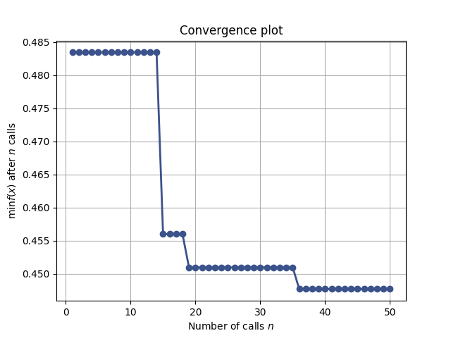
<Axes: title={'center': 'Convergence plot'}, xlabel='Number of calls $n$', ylabel='$\\min f(x)$ after $n$ calls'>