Note
Go to the end to download the full example code or to run this example in your browser via Binder
Bayesian optimization with skopt#
Gilles Louppe, Manoj Kumar July 2016. Reformatted by Holger Nahrstaedt 2020
Problem statement#
We are interested in solving
under the constraints that
\(f\) is a black box for which no closed form is known (nor its gradients);
\(f\) is expensive to evaluate;
and evaluations of \(y = f(x)\) may be noisy.
Disclaimer. If you do not have these constraints, then there is certainly a better optimization algorithm than Bayesian optimization.
This example uses plots.plot_gaussian_process which is available
since version 0.8.
Bayesian optimization loop#
For \(t=1:T\):
Given observations \((x_i, y_i=f(x_i))\) for \(i=1:t\), build a probabilistic model for the objective \(f\). Integrate out all possible true functions, using Gaussian process regression.
optimize a cheap acquisition/utility function \(u\) based on the posterior distribution for sampling the next point. \(x_{t+1} = arg \\min_x u(x)\) Exploit uncertainty to balance exploration against exploitation.
Sample the next observation \(y_{t+1}\) at \(x_{t+1}\).
Acquisition functions#
Acquisition functions \(u(x)\) specify which sample \(x\): should be tried next:
Expected improvement (default): \(-EI(x) = -\\mathbb{E} [f(x) - f(x_t^+)]\)
Lower confidence bound: \(LCB(x) = \\mu_{GP}(x) + \\kappa \\sigma_{GP}(x)\)
Probability of improvement: \(-PI(x) = -P(f(x) \\geq f(x_t^+) + \\kappa)\)
where \(x_t^+\) is the best point observed so far.
In most cases, acquisition functions provide knobs (e.g., \(\\kappa\)) for controlling the exploration-exploitation trade-off. - Search in regions where \(\\mu_{GP}(x)\) is high (exploitation) - Probe regions where uncertainty \(\\sigma_{GP}(x)\) is high (exploration)
print(__doc__)

import numpy as np

np.random.seed(237)
import matplotlib.pyplot as plt

from skopt.plots import plot_gaussian_process
Toy example#
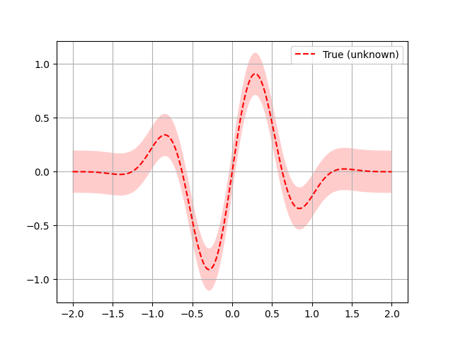
Let assume the following noisy function \(f\):
noise_level = 0.1


def f(x, noise_level=noise_level):
    return np.sin(5 * x[0]) * (1 - np.tanh(x[0] ** 2)) + np.random.randn() * noise_level
Note. In skopt, functions \(f\) are assumed to take as input a 1D
vector \(x\): represented as an array-like and to return a scalar
\(f(x)\):.
# Plot f(x) + contours
x = np.linspace(-2, 2, 400).reshape(-1, 1)
fx = [f(x_i, noise_level=0.0) for x_i in x]
plt.plot(x, fx, "r--", label="True (unknown)")
plt.fill(
    np.concatenate([x, x[::-1]]),
    np.concatenate(
        (
            [fx_i - 1.9600 * noise_level for fx_i in fx],
            [fx_i + 1.9600 * noise_level for fx_i in fx[::-1]],
        )
    ),
    alpha=0.2,
    fc="r",
    ec="None",
)
plt.legend()
plt.grid()
plt.show()
Bayesian optimization based on gaussian process regression is implemented in
gp_minimize and can be carried out as follows:
from skopt import gp_minimize

res = gp_minimize(
    f,  # the function to minimize
    [(-2.0, 2.0)],  # the bounds on each dimension of x
    acq_func="EI",  # the acquisition function
    n_calls=15,  # the number of evaluations of f
    n_random_starts=5,  # the number of random initialization points
    noise=0.1**2,  # the noise level (optional)
    random_state=1234,
)  # the random seed
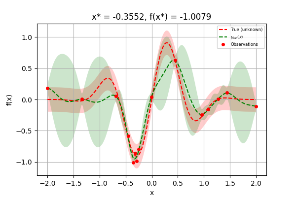
Accordingly, the approximated minimum is found to be:
f"x^*={res.x[0]:.4f}, f(x^*)={res.fun:.4f}"
'x^*=-0.3552, f(x^*)=-1.0079'
For further inspection of the results, attributes of the res named tuple
provide the following information:
x[float]: location of the minimum.fun[float]: function value at the minimum.models: surrogate models used for each iteration.x_iters[array]: location of function evaluation for each iteration.func_vals[array]: function value for each iteration.space[Space]: the optimization space.specs[dict]: parameters passed to the function.
print(res)
         fun: -1.007919274002016
           x: [-0.35518414273753307]
   func_vals: [ 3.716e-02  6.739e-03 ...  8.157e-03 -7.976e-01]
     x_iters: [[-0.009345334109402526], [1.2713537644662787], [0.4484475787090836], [1.0854396754496047], [1.4426790855107496], [0.9579248468740365], [-0.4515808656811222], [-0.6859481043850504], [-0.35518414273753307], [-0.29315377717222235], [-0.32099415298782463], [-2.0], [2.0], [-1.3373742019079444], [-0.24784228664930108]]
      models: [GaussianProcessRegressor(kernel=1**2 * Matern(length_scale=1, nu=2.5) + WhiteKernel(noise_level=0.01),
                                       n_restarts_optimizer=2, noise=0.010000000000000002,
                                       normalize_y=True, random_state=822569775), GaussianProcessRegressor(kernel=1**2 * Matern(length_scale=1, nu=2.5) + WhiteKernel(noise_level=0.01),
                                       n_restarts_optimizer=2, noise=0.010000000000000002,
                                       normalize_y=True, random_state=822569775), GaussianProcessRegressor(kernel=1**2 * Matern(length_scale=1, nu=2.5) + WhiteKernel(noise_level=0.01),
                                       n_restarts_optimizer=2, noise=0.010000000000000002,
                                       normalize_y=True, random_state=822569775), GaussianProcessRegressor(kernel=1**2 * Matern(length_scale=1, nu=2.5) + WhiteKernel(noise_level=0.01),
                                       n_restarts_optimizer=2, noise=0.010000000000000002,
                                       normalize_y=True, random_state=822569775), GaussianProcessRegressor(kernel=1**2 * Matern(length_scale=1, nu=2.5) + WhiteKernel(noise_level=0.01),
                                       n_restarts_optimizer=2, noise=0.010000000000000002,
                                       normalize_y=True, random_state=822569775), GaussianProcessRegressor(kernel=1**2 * Matern(length_scale=1, nu=2.5) + WhiteKernel(noise_level=0.01),
                                       n_restarts_optimizer=2, noise=0.010000000000000002,
                                       normalize_y=True, random_state=822569775), GaussianProcessRegressor(kernel=1**2 * Matern(length_scale=1, nu=2.5) + WhiteKernel(noise_level=0.01),
                                       n_restarts_optimizer=2, noise=0.010000000000000002,
                                       normalize_y=True, random_state=822569775), GaussianProcessRegressor(kernel=1**2 * Matern(length_scale=1, nu=2.5) + WhiteKernel(noise_level=0.01),
                                       n_restarts_optimizer=2, noise=0.010000000000000002,
                                       normalize_y=True, random_state=822569775), GaussianProcessRegressor(kernel=1**2 * Matern(length_scale=1, nu=2.5) + WhiteKernel(noise_level=0.01),
                                       n_restarts_optimizer=2, noise=0.010000000000000002,
                                       normalize_y=True, random_state=822569775), GaussianProcessRegressor(kernel=1**2 * Matern(length_scale=1, nu=2.5) + WhiteKernel(noise_level=0.01),
                                       n_restarts_optimizer=2, noise=0.010000000000000002,
                                       normalize_y=True, random_state=822569775), GaussianProcessRegressor(kernel=1**2 * Matern(length_scale=1, nu=2.5) + WhiteKernel(noise_level=0.01),
                                       n_restarts_optimizer=2, noise=0.010000000000000002,
                                       normalize_y=True, random_state=822569775)]
       space: Space([Real(low=-2.0, high=2.0, prior='uniform', transform='normalize')])
random_state: RandomState(MT19937)
       specs:     args:                    func: <function f at 0x0000020BD78EB060>
                                     dimensions: Space([Real(low=-2.0, high=2.0, prior='uniform', transform='normalize')])
                                 base_estimator: GaussianProcessRegressor(kernel=1**2 * Matern(length_scale=1, nu=2.5),
                                                                          n_restarts_optimizer=2, noise=0.010000000000000002,
                                                                          normalize_y=True, random_state=822569775)
                                        n_calls: 15
                                n_random_starts: 5
                               n_initial_points: 10
                        initial_point_generator: random
                                       acq_func: EI
                                  acq_optimizer: auto
                                             x0: None
                                             y0: None
                                   random_state: RandomState(MT19937)
                                        verbose: False
                                       callback: None
                                       n_points: 10000
                           n_restarts_optimizer: 5
                                             xi: 0.01
                                          kappa: 1.96
                                         n_jobs: 1
                               model_queue_size: None
                               space_constraint: None
              function: base_minimize
Together these attributes can be used to visually inspect the results of the minimization, such as the convergence trace or the acquisition function at the last iteration:
from skopt.plots import plot_convergence

plot_convergence(res)
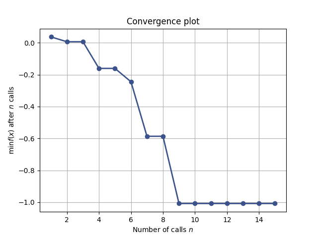
<Axes: title={'center': 'Convergence plot'}, xlabel='Number of calls $n$', ylabel='$\\min f(x)$ after $n$ calls'>
Let us now visually examine
The approximation of the fit gp model to the original function.
The acquisition values that determine the next point to be queried.
plt.rcParams["figure.figsize"] = (8, 14)


def f_wo_noise(x):
    return f(x, noise_level=0)
Plot the 5 iterations following the 5 random points
for n_iter in range(5):
    # Plot true function.
    plt.subplot(5, 2, 2 * n_iter + 1)

    if n_iter == 0:
        show_legend = True
    else:
        show_legend = False

    ax = plot_gaussian_process(
        res,
        n_calls=n_iter,
        objective=f_wo_noise,
        noise_level=noise_level,
        show_legend=show_legend,
        show_title=False,
        show_next_point=False,
        show_acq_func=False,
    )
    ax.set_ylabel("")
    ax.set_xlabel("")
    # Plot EI(x)
    plt.subplot(5, 2, 2 * n_iter + 2)
    ax = plot_gaussian_process(
        res,
        n_calls=n_iter,
        show_legend=show_legend,
        show_title=False,
        show_mu=False,
        show_acq_func=True,
        show_observations=False,
        show_next_point=True,
    )
    ax.set_ylabel("")
    ax.set_xlabel("")

plt.show()
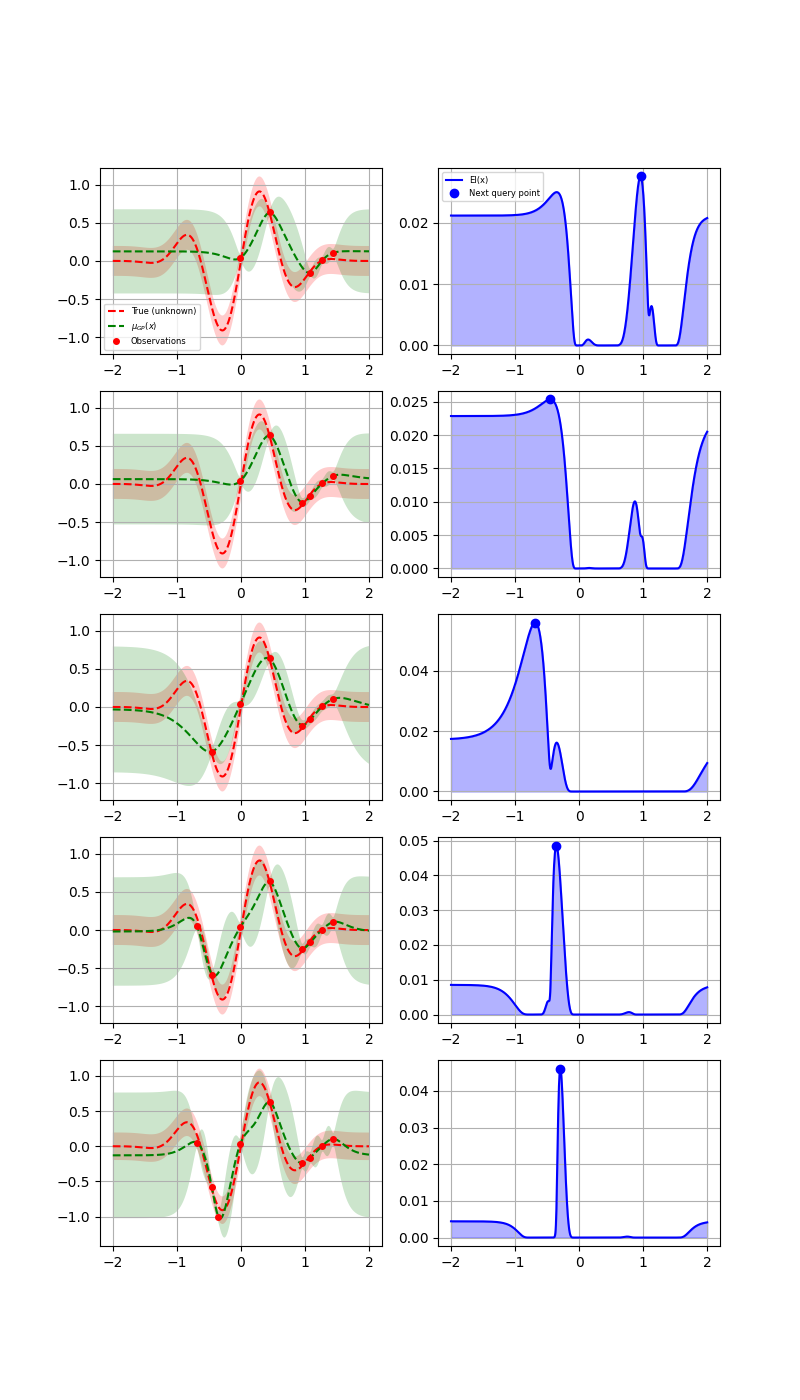
The first column shows the following:
The true function.
The approximation to the original function by the gaussian process model
How sure the GP is about the function.
The second column shows the acquisition function values after every surrogate model is fit. It is possible that we do not choose the global minimum but a local minimum depending on the minimizer used to minimize the acquisition function.
At the points closer to the points previously evaluated at, the variance dips to zero.
Finally, as we increase the number of points, the GP model approaches the actual function. The final few points are clustered around the minimum because the GP does not gain anything more by further exploration:
plt.rcParams["figure.figsize"] = (6, 4)

# Plot f(x) + contours
_ = plot_gaussian_process(res, objective=f_wo_noise, noise_level=noise_level)

plt.show()
Total running time of the script: (0 minutes 3.907 seconds)