Comparing initial sampling methods

Holger Nahrstaedt 2020 Sigurd Carlsen October 2019

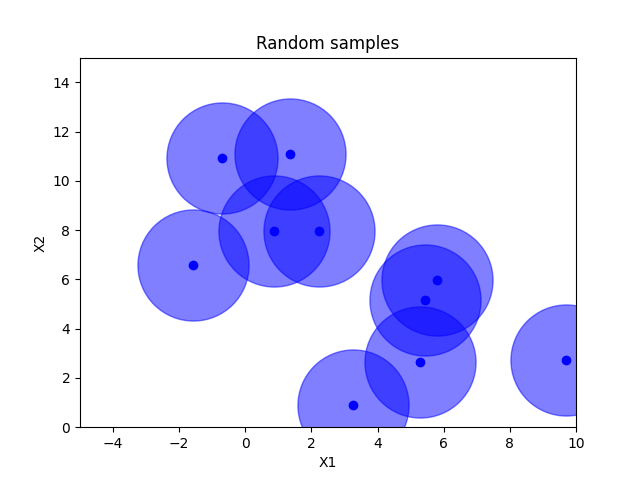
When doing baysian optimization we often want to reserve some of the early part of the optimization to pure exploration. By default the optimizer suggests purely random samples for the first n_initial_points (10 by default). The downside to this is that there is no guarantee that these samples are spread out evenly across all the dimensions.

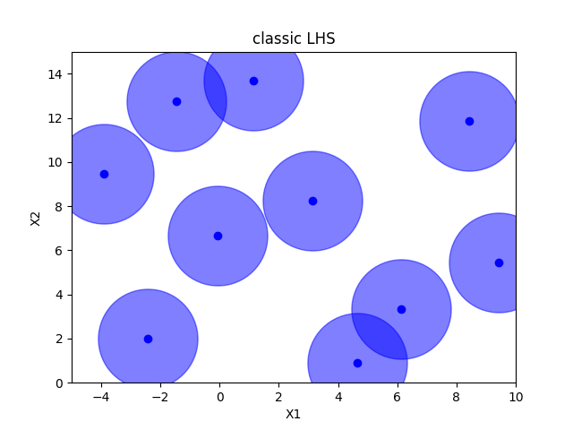
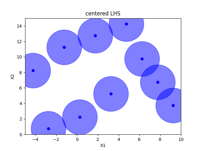
Sampling methods as Latin hypercube, Sobol’, Halton and Hammersly take advantage of the fact that we know beforehand how many random points we want to sample. Then these points can be “spread out” in such a way that each dimension is explored.

See also the example on an integer space sphx_glr_auto_examples_initial_sampling_method_integer.py

print(__doc__)
import numpy as np

np.random.seed(123)
import matplotlib.pyplot as plt
from scipy.spatial.distance import pdist

from skopt.sampler import Grid, Halton, Hammersly, Lhs, Sobol
from skopt.space import Space

def plot_searchspace(x, title):
    fig, ax = plt.subplots()
    plt.plot(np.array(x)[:, 0], np.array(x)[:, 1], 'bo', label='samples')
    plt.plot(np.array(x)[:, 0], np.array(x)[:, 1], 'bo', markersize=80, alpha=0.5)
    # ax.legend(loc="best", numpoints=1)
    ax.set_xlabel("X1")
    ax.set_xlim([-5, 10])
    ax.set_ylabel("X2")
    ax.set_ylim([0, 15])
    plt.title(title)


n_samples = 10

space = Space([(-5.0, 10.0), (0.0, 15.0)])
# space.set_transformer("normalize")

Random sampling

x = space.rvs(n_samples)
plot_searchspace(x, "Random samples")
pdist_data = []
x_label = []
pdist_data.append(pdist(x).flatten())
x_label.append("random")

Sobol’

sobol = Sobol()
x = sobol.generate(space.dimensions, n_samples)
plot_searchspace(x, "Sobol'")
pdist_data.append(pdist(x).flatten())
x_label.append("sobol'")

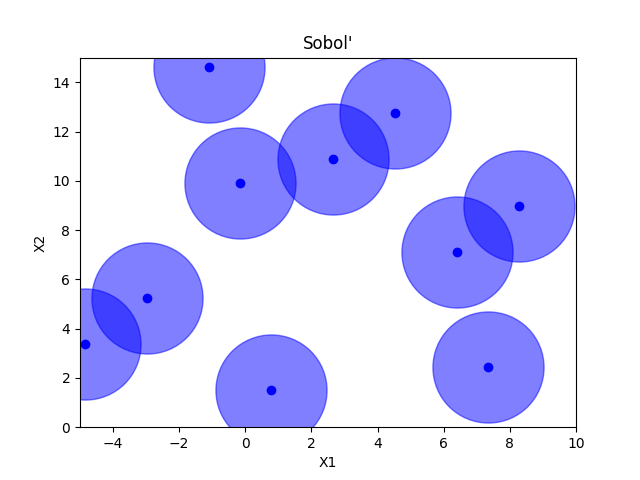
D:\git\scikit-optimize\skopt\sampler\sobol.py:521: UserWarning: The balance properties of Sobol' points require n to be a power of 2. 0 points have been previously generated, then: n=0+10=10.
  warnings.warn(

Classic Latin hypercube sampling

lhs = Lhs(lhs_type="classic", criterion=None)
x = lhs.generate(space.dimensions, n_samples)
plot_searchspace(x, 'classic LHS')
pdist_data.append(pdist(x).flatten())
x_label.append("lhs")

Centered Latin hypercube sampling

lhs = Lhs(lhs_type="centered", criterion=None)
x = lhs.generate(space.dimensions, n_samples)
plot_searchspace(x, 'centered LHS')
pdist_data.append(pdist(x).flatten())
x_label.append("center")

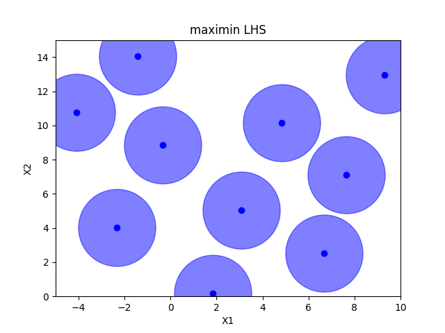
Maximin optimized hypercube sampling

lhs = Lhs(criterion="maximin", iterations=10000)
x = lhs.generate(space.dimensions, n_samples)
plot_searchspace(x, 'maximin LHS')
pdist_data.append(pdist(x).flatten())
x_label.append("maximin")

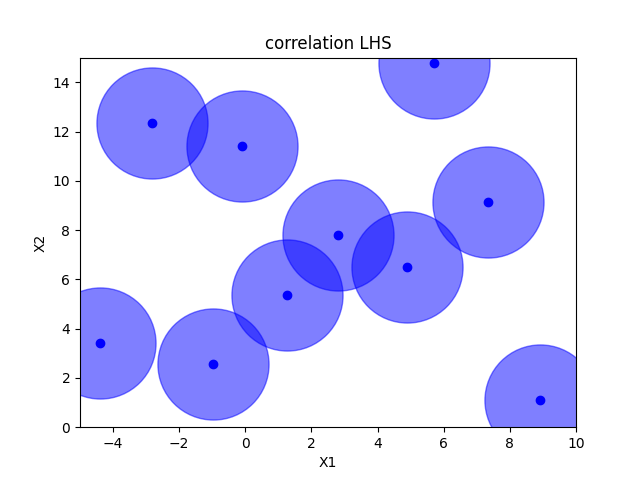
Correlation optimized hypercube sampling

lhs = Lhs(criterion="correlation", iterations=10000)
x = lhs.generate(space.dimensions, n_samples)
plot_searchspace(x, 'correlation LHS')
pdist_data.append(pdist(x).flatten())
x_label.append("corr")

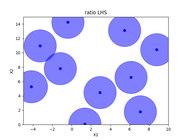
Ratio optimized hypercube sampling

lhs = Lhs(criterion="ratio", iterations=10000)
x = lhs.generate(space.dimensions, n_samples)
plot_searchspace(x, 'ratio LHS')
pdist_data.append(pdist(x).flatten())
x_label.append("ratio")

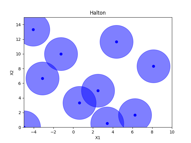
Halton sampling

halton = Halton()
x = halton.generate(space.dimensions, n_samples)
plot_searchspace(x, 'Halton')
pdist_data.append(pdist(x).flatten())
x_label.append("halton")

Hammersly sampling

hammersly = Hammersly()
x = hammersly.generate(space.dimensions, n_samples)
plot_searchspace(x, 'Hammersly')
pdist_data.append(pdist(x).flatten())
x_label.append("hammersly")

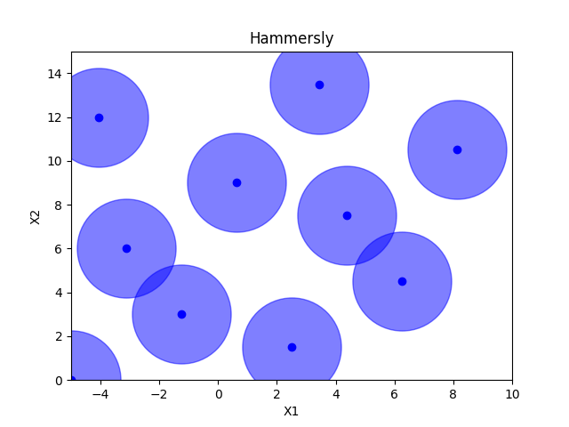
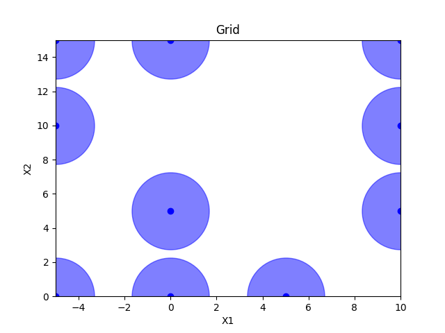
Grid sampling

grid = Grid(border="include", use_full_layout=False)
x = grid.generate(space.dimensions, n_samples)
plot_searchspace(x, 'Grid')
pdist_data.append(pdist(x).flatten())
x_label.append("grid")

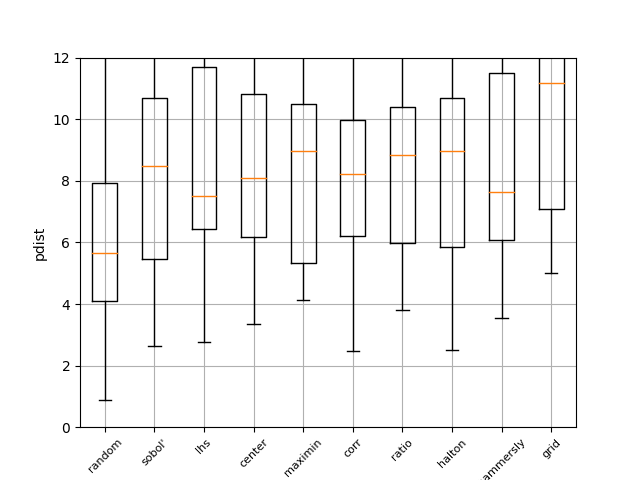
Pdist boxplot of all methods

This boxplot shows the distance between all generated points using Euclidian distance. The higher the value, the better the sampling method. It can be seen that random has the worst performance

fig, ax = plt.subplots()
ax.boxplot(pdist_data)
plt.grid(True)
plt.ylabel("pdist")
_ = ax.set_ylim(0, 12)
_ = ax.set_xticklabels(x_label, rotation=45, fontsize=8)